23. Some more math
This section is given as bonus material and is not mandatory. If you are curious how we derived the final accumulative equation for BPTT, this section will help you out.
In the previous videos, we talked about Backpropagation Through Time. We used a lot of partial derivatives, accumulating the contributions to the change in the error from each state. Remember?
When we needed a general scheme for the BPTT, I simply displayed the equation without giving you further explanations.
As a reminder, the following two equations were derived when adjusting the weights of matrix W_s and matrix W_x:
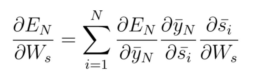
Equation 48: BPTT calculations for the purpose of adjusting Ws
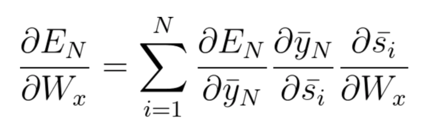
Equation 49: BPTT calculations for the purpose of adjusting Wx
To generalize the case, we will avoid proving equation 48 or 49, and will focus on a general framework.
Let's look at the following sketch, presenting a portion of a network:
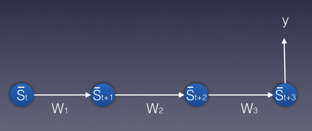
In the picture above, we have four states, starting with s_t.
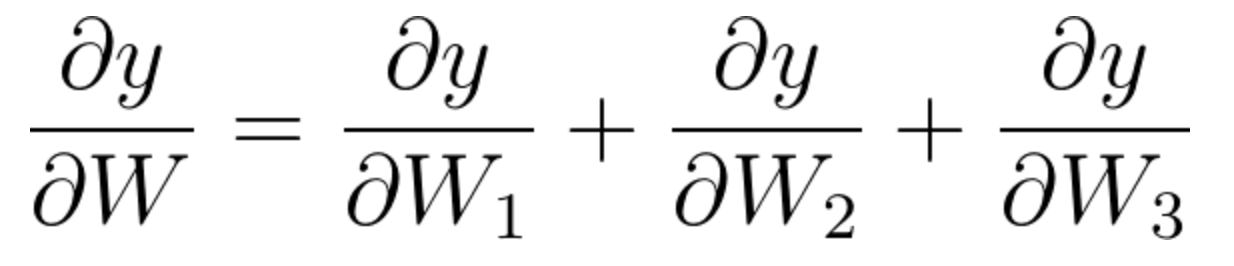
We will initially consider the three weight matrices W_1,W_2 and W_3 as three different matrices.
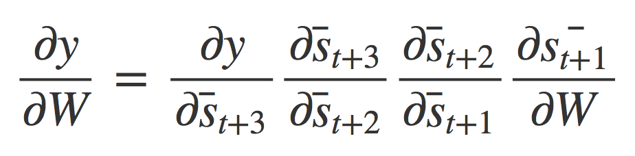
Using the chain rule we can derive the following three equations:
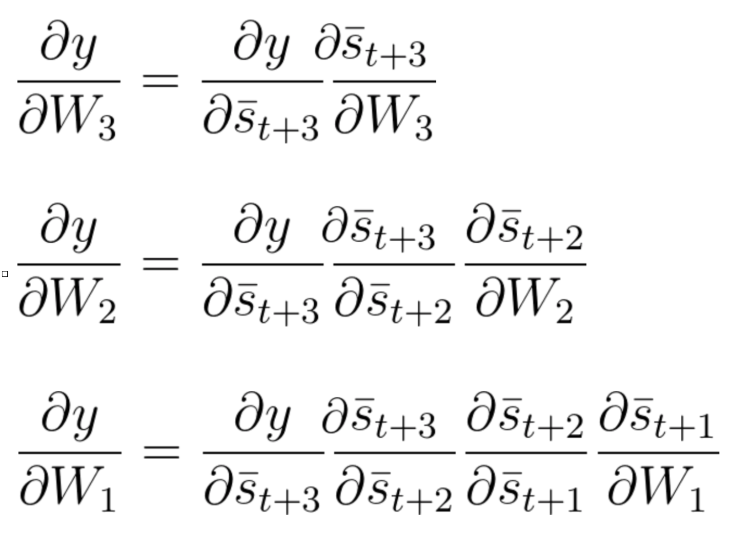
Equation 50 (Equation set)
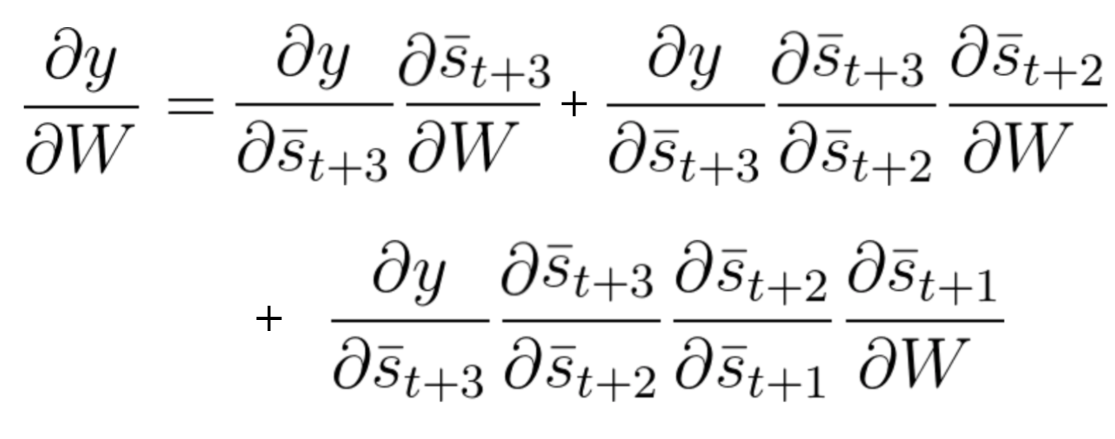
In Backpropagation Through Time we accumulate the contributions, therefore:
Equation 51
Since this network is displayed as unfolded in time, we understand that the weight matrices connecting each of the states are identical. Therefore:
W_1=W_2=W_3
Lets simply call it weight matrix W. Therefore:
W_1=W_2=W_3=W
Equation 52
From equation 52, equation 51 and the set of equations 50 we derive that:
Equation 52
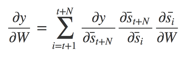
Equation 52 summarizes the mathematical procedure of BPTT and can be simply written as:
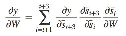
Equation 53
Notice that for i=t+1, we derive the following:
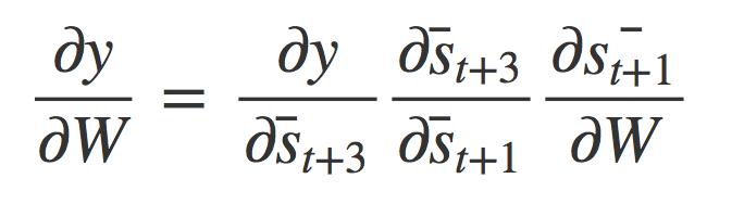
Equation 54
With the use of the chain rule we can derive the following equation (displayed in set of equations 50).
Equation 55
A general derivation of the BPTT calculation can be displayed the following way:
Equation 55